Kaggle time series question
After the first exercise I was keen on exploring it a little bit more and I played around at the end of the notebook.
I performed the regression with the lag_1 and time feature together and added
another feature called diff, the difference between lag_1 and time .
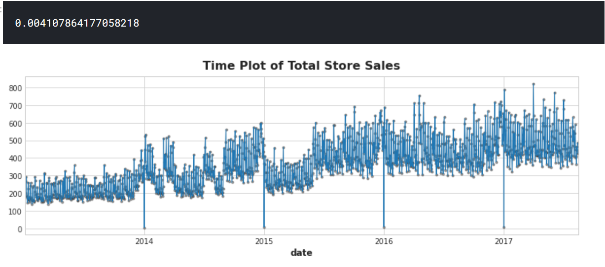
Then I discovered, that the prediction is kind of “perfect”, so I started to reduce the amount of days in the fitting of the model. And it seems, that with only four (!) days in the model fit the sales prediction becomes kind of “perfect”.
Can somebody explain what happened here, because I don’t understand it? The “forecast” even got the zero sales at new year’s eve, which seems quite astonishing.
I’ve linked my notebook, but here is the questionable part:
df = average_sales.to_frame()

# Create a time dummy
time = np.arange(len(df))
df['time'] = time # add to dataframe

# Create a lag feature from the target 'sales'
lag_1 = df['sales'].shift(1)
df['lag_1'] = lag_1  # add to dataframe

# Create a diff feature from the target 'sales'
diff = df['sales'].diff()
df['diff'] = diff  # add to dataframe

X = df.loc[:, ['time', 'lag_1', 'diff']].dropna()  # features
y = df.loc[:, 'sales']  # target
y, X = y.align(X, join='inner')  # drop corresponding values in target

# YOUR CODE HERE: Create a LinearRegression instance and fit it to X and y.
model = LinearRegression()
model.fit(X[0:4], y[0:4])

# YOUR CODE HERE: Create Store the fitted values as a time series with
# the same time index as the training data
y_pred = pd.Series(model.predict(X), index=X.index)

ax = y.plot(**plot_params, alpha=0.5)
ax = y_pred.plot(ax=ax, linewidth=1)
ax.set_title('Time Plot of Total Store Sales');
max(abs(y-y_pred))
Here is the output of the code above: